That cost pressure is mounting. Gartner forecasts worldwide public cloud spending at $723.4 billion in 2025, up 21.5% from 2024. Meanwhile, 72% of companies already exceeded their cloud budget in the most recent fiscal year. Query inefficiency is a direct contributor to both figures.
The good news: poor query performance is rarely a hardware problem. It's almost always a design problem. This article breaks down the highest-impact optimization techniques — from SQL rewrites to schema architecture, indexing, and pipeline hygiene — across modern cloud warehouses like Snowflake, BigQuery, and Redshift.
Key Takeaways
- Writing leaner SQL (avoiding
SELECT *, filtering early) reduces I/O costs immediately with no schema changes required - Partitioning large tables and using materialized views cut the volume of data scanned per query
- Star schema design reduces join complexity; SQL tuning alone can't fix a poorly structured schema
- ETL/ELT hygiene (batch loads, proper file sizing) prevents fragmentation that degrades scan performance over time
- Auto-maintained statistics work well in most cloud warehouses, though large bulk loads may still need a manual refresh
What Is Data Warehouse Query Optimization?
Data warehouse query optimization is the practice of improving query execution speed, reducing compute resource consumption, and increasing analytical throughput — applied across multiple layers: SQL code, schema design, indexing, storage organization, and pipeline architecture.
It's distinct from traditional OLTP database tuning. Where OLTP workloads involve many small, concurrent read/write transactions, data warehouses handle large-volume, read-heavy analytical queries across millions or billions of rows. The performance dynamics are different, and so are the solutions.
How the Query Optimizer Works
Every modern cloud warehouse generates an execution plan before running a query. The optimizer evaluates the query's structure, available statistics (row counts, column cardinality, data distribution), and physical data layout to determine the most efficient retrieval path.
When the optimizer lacks accurate information, it makes suboptimal choices. Common failure modes include:
- Full table scans instead of partition pruning
- Inefficient join ordering due to missing row count statistics
- Unnecessary data movement across compute nodes from fragmented storage
These failures compound over time. As data volumes grow, query patterns shift, and schemas evolve, plans that once performed well can quietly degrade — making optimization an ongoing responsibility, not a one-time fix.
Key SQL & Query-Level Optimization Techniques
This is the most immediately actionable layer — these are changes you can often make to existing queries without touching warehouse architecture. Small SQL rewrites frequently produce significant execution plan improvements.
Write Leaner SELECT Statements
Avoid SELECT *. In columnar storage systems like Snowflake, BigQuery, and Redshift, data is organized by column — meaning the engine only reads the columns you actually request. SELECT * forces it to read every column, negating that advantage entirely and inflating I/O, memory consumption, and (in BigQuery's case) direct query costs.
Specifying only the columns you need is the simplest query change with the most immediate impact on I/O and cost.
Filter Early with WHERE Clauses
Apply filters as early as possible — ideally before JOINs and aggregations — to reduce the number of rows processed at every subsequent step.
Modern query optimizers support predicate pushdown: the ability to push filter logic down to the storage layer, skipping irrelevant data files or row groups before they're ever loaded into memory. Snowflake's pushdown optimization filters unneeded rows "as early as possible during query processing," reducing both processing time and memory overhead.
Optimize JOIN Logic
Join performance depends on:
- Joining on indexed or clustered columns where possible
- Filtering dimension tables before joining them to fact tables
- Choosing the right join type: hash joins handle large unsorted datasets well; nested loop joins are better suited to small lookup tables
In most cases, reducing intermediate result set sizes before a join delivers more gains than tuning join mechanics after the fact.
Use Materialized Views for Pre-Aggregated Results
Materialized views store pre-computed query results — useful when the same expensive aggregation or multi-table join runs repeatedly. Rather than re-executing the full query each time, the warehouse serves results from the stored view.
They work best for stable, frequently-run analytical queries. The main tradeoff is refresh overhead and additional storage cost. Platform behavior differs here:
- BigQuery: handles incremental refresh automatically at no extra charge
- Snowflake: bills materialized view maintenance as credits on Enterprise Edition
Use Query Caching
Cloud warehouses cache query results and re-serve them for identical subsequent queries without re-executing:
| Platform | Cache Duration | Cost of Cache Hit |
|---|---|---|
| Snowflake | 24 hours (resets on reuse, up to 31 days) | Zero warehouse credits |
| BigQuery | ~24 hours | No charge |
| Redshift | Session-level, leader node | No compute node processing |
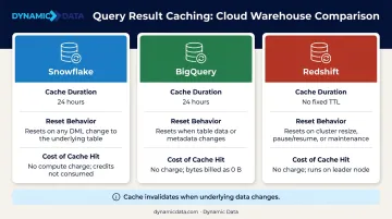
Caching is most valuable for repeated dashboard loads and scheduled reports. Cache invalidation occurs when underlying data changes, so it's less effective for real-time or frequently updated tables.
Schema Design & Data Modeling for Performance
Schema design is the architectural foundation that determines how efficiently the query engine navigates data. Poor schema choices force unnecessary joins, inflate scans, and produce inefficient execution plans — problems that SQL tuning alone can't solve once the structure is set.
Star Schema vs. Snowflake Schema
The choice between these two models has a direct impact on query execution time:
- Star schema: Denormalized structure with dimension tables directly connected to the fact table. Fewer joins, faster analytical queries, aligns well with how MPP engines distribute and process data.
- Snowflake schema: Normalized structure with dimensions broken into sub-dimensions. More storage-efficient, but requires additional joins that slow analytical reads.
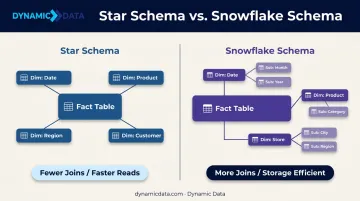
For analytical workloads where read speed matters more than write efficiency, star schema is generally preferred. Redshift's distribution key guidance, for example, explicitly recommends co-locating fact and dimension tables on join columns to minimize cross-node data movement.
Schema choice shapes everything downstream — including how you design the individual tables within it.
Fact and Dimension Table Design Principles
Fact tables store measurable events at the most granular level — transactions, clicks, sensor readings. Dimension tables store the descriptive context that gives those events meaning: customers, products, dates, locations.
Getting both right reduces scan volume and speeds up aggregations. Key design principles:
- Keep fact tables narrow — include foreign keys and numeric measures, not descriptive attributes
- Use surrogate keys (integer-based) on dimension tables rather than natural keys for faster joins
- Apply slowly changing dimension (SCD) strategies deliberately — SCD Type 1 for overwrite, Type 2 for history, based on your reporting needs
- Avoid storing pre-aggregated data in fact tables unless query patterns consistently demand it