

We Tried BigQuery Measures: A Semantic Layer That Lives Inside a Graph
Most data teams have sat through some version of the same meeting. Finance brings one revenue number, marketing's dashboard shows another, and the meeting turns into a debate about whose figure is right. The KPI lives in too many places: a SQL view, a calculated field in one report, a filter someone added to another. Each copy drifted a little. Now AI agents are asking the same questions, and when the definition isn't written down they guess, giving "confident but sometimes wrong answers". A semantic layer exists to end that meeting: define each metric once, in one place, and let every dashboard, query, and agent ask for it by name.
On November 10, 2026, Google made BigQuery measures generally available. Measures are metrics you declare once, inside BigQuery. Each one's aggregation is locked to the key of its table, so it stays correct even when a join duplicates rows. The twist is where they live. There's no separate semantic layer product: measures sit on a BigQuery property graph, so the object that holds your metrics is also a graph you can traverse.
We built one on Google's own sample data, connected it to Data Studio, and then tried to break it. Here's how it's put together, what we learned along the way, and where we think it fits next to the semantic layers you may already use.
Your Semantic Model Is a Graph Now
If you haven't used BigQuery Graph, here's the idea. A property graph models your existing tables as entities and the relationships between them. Tables that hold entities, such as labels, artists, or songs, become nodes. The relationships between them, such as the label an artist is signed to, become edges, usually on the same foreign keys you'd join on. It doesn't copy data; it sits on top of your tables or views. In our test, it showed up in the dataset as one more object, named like a table (`music.BelenGraph`).
A measure is a metric you attach to one of those nodes: total streams on the song node, marketing budget on the label node. You declare it once, wrapped in `MEASURE()`. Unlike a regular aggregate, its calculation is tied to the key of the node it's defined on. Because the streams measure is tied to `song_id`, BigQuery counts each song once, even when a query joins songs to playlists and repeats rows. Google calls these measures "grain-locked". A measure can use `SUM`, `AVG`, `COUNT`, `MIN`, or `MAX`, or build on other measures of the same node. Window functions, `GROUP BY`, and subqueries aren't allowed inside one.
The whole model is one SQL statement, `CREATE PROPERTY GRAPH`, with a block for nodes and a block for edges. We wrote ours by hand, and in SQL there's no adding one node at a time. Every change meant re-running the whole `CREATE OR REPLACE`. The visual modeler, still in Preview, lets you add or edit nodes one by one and generates that statement for you.
Getting numbers out takes one function and one wrapper. `GRAPH_EXPAND` turns the graph back into a single wide table, joining each node to the next, with columns named after the node and the property (`Songs_streams`). Then you wrap each measure in `AGG()`, which calculates it once per key instead of once per row. The same graph can also be queried with GQL, the ISO-standard graph query language, which answers questions about connections: which songs share a playlist, which label an artist belongs to. GQL can't read measures, though.
Measures had been in Preview since April 22, 2026. The GA release adds measures that build on other measures and queries across several fact tables. It also brings custom metadata for natural-language tools, a Data Studio connector, and automatic listing in Knowledge Catalog. Looker's option to turn an Explore into a BigQuery graph is still in Preview.
One practical check before you start: measures run on on-demand pricing or the Enterprise editions, not on Standard, and GQL has the same options.
Building One, and the Three Rules We Learned the Hard Way
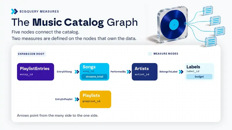
We used the music catalog from Google's measures codelab. It has five small tables: a label signs artists, an artist releases songs, and a song lands on playlists through a junction table, `PlaylistEntries`. It's tiny on purpose. One song sits on four playlists, and that's the whole trap. Our full graph has five nodes and four edges. Here's the part that matters:
```sql
CREATE OR REPLACE PROPERTY GRAPH music.BelenGraph
NODE TABLES (
music.Labels AS Labels KEY (label_id)
PROPERTIES (label_id, label_name, marketing_budget,
MEASURE(SUM(marketing_budget)) AS budget),
music.Songs AS Songs KEY (song_id)
PROPERTIES (song_id, title, artist_id, streams,
MEASURE(SUM(streams)) AS streams_total),
music.PlaylistEntries AS PlaylistEntries KEY (entry_id)
PROPERTIES (entry_id, playlist_id, song_id)
-- ...plus Artists and Playlists
)
EDGE TABLES (
music.PlaylistEntries AS EntryOfSong KEY (entry_id)
SOURCE KEY (entry_id) REFERENCES PlaylistEntries (entry_id)
DESTINATION KEY (song_id) REFERENCES Songs (song_id)
NO PROPERTIES
-- ...plus EntryInPlaylist, PerformedBy, and BelongsToLabel
);
SELECT Labels_label_name,
SUM(Songs_streams) AS with_sum, -- inflated
AGG(Songs_streams_total) AS with_agg -- counted once per song
FROM GRAPH_EXPAND("music.BelenGraph")
GROUP BY Labels_label_name;
```
The first rule: a measure works on properties, not raw columns. Our first attempt declared `MEASURE(SUM(marketing_budget))` without listing `marketing_budget` as a property. The console rejected it: "Columns are not supported in graph measure property expressions." Once we listed the column as a property too, it ran. Google's examples always do the same thing: `budget` appears in the property list and again inside the measure.
The second rule is about direction. We wrote every edge from the many side to the one side: entry to song, song to artist, artist to label. That's how the GA blog and the codelab write them too. What `GRAPH_EXPAND` cares about is the root, the table it starts from, which needs a many-to-one relationship with every node it shares an edge with. In our graph, that root is `PlaylistEntries`.
The third rule is the one that surprised us. A many-to-many table can't just be an edge. Model `PlaylistEntries` as an edge between songs and playlists and `GRAPH_EXPAND` ignores it as ambiguous. If every edge gets ignored, the call fails. The fix is to promote the junction table to a node with two many-to-one edges, one to each side, defined on the same physical table. That's why `PlaylistEntries` shows up three times in our graph: once as a node and twice as an edge.
Two smaller things cost us time. An empty `EDGE TABLES ( )` block throws a syntax error, so leave it out until you have edges. And changing the graph doesn't invalidate cached results for `GRAPH_EXPAND` queries, so turn off cached results while you iterate, or you'll be staring at an old number.
What Happened When We Ran It
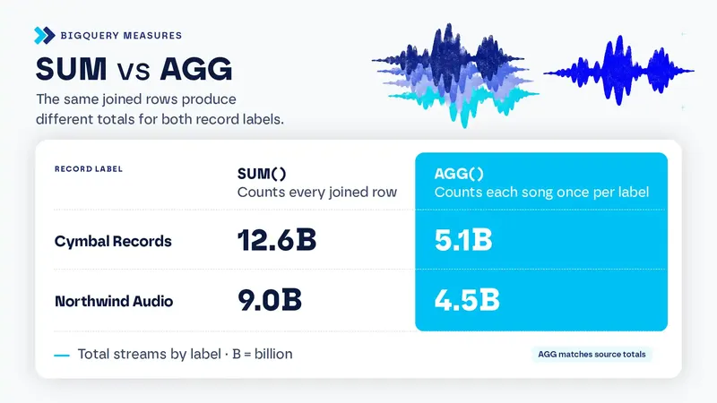
The first query did exactly what the docs promised. Grouped by label, `SUM` over the flattened table returned 12.6 billion streams for Cymbal Records and 9.0 billion for Northwind Audio. `AGG` returned 5.1 billion and 4.5 billion, which match the source tables. The label budget, two hops away from the root, behaved the same way. Cymbal appears on eight rows, so a plain `SUM` gave it 40 million, while the measure gave 5 million. Grain locking works for a dimension attribute, not only for a fact.
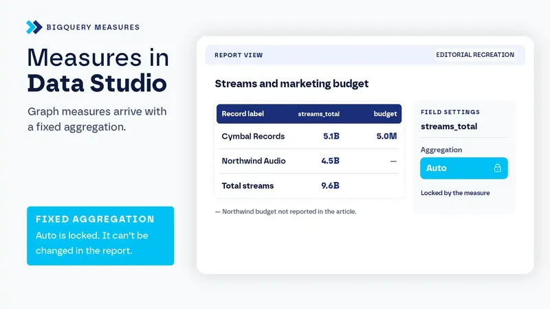
Data Studio was the part we were most curious about, because that's where most of our clients would see these numbers. The BigQuery connector lists graphs next to tables and asks for a start node. Measures arrive as metrics with a fixed aggregation you can't change. In our report it showed as "Auto," locked. In our test, a table by label returned the same values as `AGG` in SQL, and a scorecard showed 9.6 billion rather than an inflated total. A filter on one playlist kept the grain right, and a calculated field dividing streams by budget worked on the aggregated measures instead of re-adding rows. That's consistent with Google's line that Data Studio prevents "accidental client-side re-aggregations".
GQL ran on our on-demand project. Asking it for a measure failed with "Property streams_total is not exposed by element type", as documented. The two modes can still meet in one query. In our test, a `GRAPH_TABLE` subquery picked the songs that share a playlist with Neon Summer. Then `GRAPH_EXPAND` with `AGG` measured only those songs: 7.6 billion streams, where a plain `SUM` said 13.6 billion. The docs don't show this combination, but it's the pattern that makes the graph worth having: GQL finds who, `AGG` counts how much.
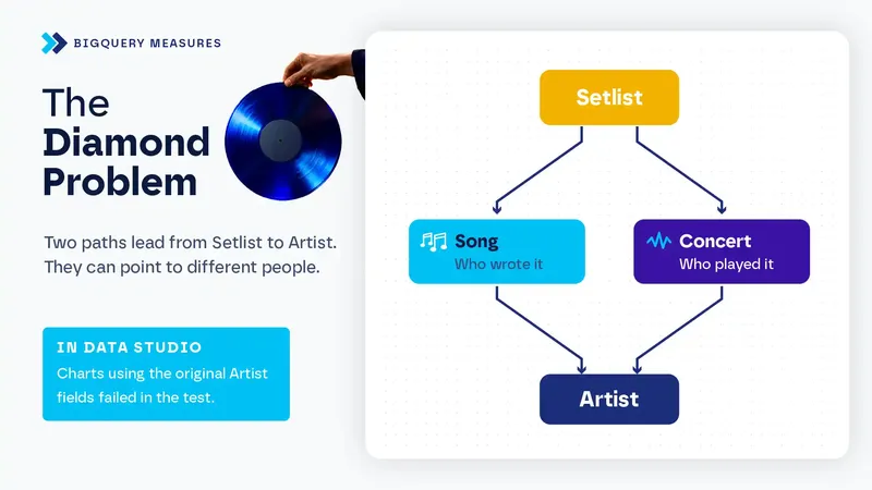
Then we gave it a harder shape. We added two fictional tables, concerts and their setlists. Now an artist could be reached from a setlist two ways: through the song (who wrote it) and through the concert (who played it). They don't always agree. One artist covered another's song. `GRAPH_EXPAND` didn't pick a path or fail. It duplicated the artist node and prefixed each copy with the edge it came through: `ConcertBy_Artists_artist_name` and `PerformedBy_Artists_artist_name`. Plain `Artists_artist_name` stopped existing. We didn't find that behavior in the docs. It's useful, and it makes edge names part of your column names, so name edges as roles.
The path you choose answers a different question. By the artist who played, ticket sales added up to 43,000. By the artist whose song was played, the rows added up to 58,000, while the total stayed at 43,000. That's the same effect as full-credit attribution in marketing. Grain locking stops double counting inside a group, not across groups. The root matters just as quietly. Data that isn't reachable from the start node doesn't appear, so from the setlist side, streams dropped to 9.2 billion because one song was never played live. There was no error.
Data Studio didn't survive the diamond. Its field list offered the unprefixed `Artists_*` fields, which no longer exist in BigQuery. Any chart using them failed with "Invalid Field Configuration." If a model has to reach Data Studio, avoid diamonds for now.
Is It Better Than Other Semantic Layers?
Not across the board. Our take: it's worth it when your whole stack is already on Google. That's a narrower answer than the launch suggests.
What no other semantic layer we know gives you is metrics and relationships in one object. The same graph answers "how much" with `AGG` and "why" with GQL. It lives in the engine, so there's no extra product to license or host. Fan-out is handled instead of forbidden: dbt's MetricFlow restricts fan-out joins, and BigQuery lets them happen and still counts correctly. The Data Studio connector respects measures natively, while the dbt Semantic Layer has no native Data Studio integration. Conversational Analytics agents can also use the measures, descriptions, and synonyms defined on a graph. We haven't tested the agent yet.
As a metrics engine, though, it's the simplest of the group. Derived measures only combine measures on the same table, and window functions aren't allowed. dbt has cumulative and conversion metrics and ratios across semantic models. Snowflake semantic views support semi-additive metrics, window-function metrics, and derived metrics across tables. With BigQuery, period over period and running totals go in the SQL you write on top.
The operational side is thinner too. As far as we could tell, there's no documented Git or CI workflow and no documented per-user security for measures. In SQL, the whole graph gets redeclared on every change. It's BigQuery only, although Spanner Graph shares the same schema. We found nothing documenting Power BI reading BigQuery measures, while the dbt Semantic Layer does integrate with Power BI. Looker's bridge into BigQuery graphs is still in Preview, ignores `access_filter` and `sql_always_where`, and needs joins that form a tree.
So use it when your data is in BigQuery, your reports are in Data Studio, and your metrics are sums, counts, and ratios that joins keep inflating. It also fits when you want an agent to answer questions that mix relationships and numbers. Skip it when you need time-based metrics, report in Power BI or Tableau, run more than one warehouse, or need role-playing dimensions to show up in Data Studio.
Want to See If It Fits Your Stack?
BigQuery measures do their best work when the tables underneath are already clean and keyed. The graph is the easy part. If you'd like help deciding whether it fits your stack, or getting your models ready for it, let's talk. Happy to walk you through how we'd approach it.
Frequently Asked Questions
Are BigQuery measures generally available? Yes. Measures went GA on November 10, 2026, after a Preview that started on April 22, 2026.
Which BigQuery edition do I need? Measures work with on-demand pricing and the Enterprise and Enterprise Plus editions, not Standard. GQL runs on on-demand pricing or an Enterprise or Enterprise Plus reservation.
Do I have to copy my data into the graph? No. A graph is defined over existing tables or views, and storage is charged once for those tables, however many graphs use them.
Can I query measures with GQL? No. GQL queries can't reference a measure. You read measures through `GRAPH_EXPAND` and `AGG()`.
Does it work with Data Studio? Yes. The BigQuery connector connects to graphs and imports measures as metrics with a fixed aggregation. In our test, a graph where one node is reachable by two paths broke the data source.
Written by Belén Rumie
Principal Consultant - Data Strategy & Platform